Telemetry Data Volume Cost Optimization in High-Scale Systems

Most engineering teams confronting an observability bill that has doubled in a quarter reach for the same explanation: they are generating more data. Three cost vectors drive the bill: volume, cardinality, and retention tier. Cardinality is the fastest-moving of the three and the least visible, and treating it as a volume problem is why the obvious fix, collecting less, so often fails to move the number.

A high-cardinality custom metric tagged with user IDs, transaction IDs, or request IDs can multiply a single metric into hundreds of millions of unique time series. On a per-series billing model, adding one high-cardinality tag to a popular metric can produce a seven-figure annual increase. A developer added a tag for debugging convenience, and the multiplication happened silently in the backend's series count.

AI workloads add a structurally new vector to this equation. Every model call, tool execution, and reasoning step must be captured as a structured span, so teams adding AI features see large multipliers on existing observability data volume. The cost consequence was never part of the design conversation.

The root issue is that OpenTelemetry instrumentation and backend pricing are separate decisions. OTel is free, but it increases signal volume through more spans and richer attributes. Per-GB backends monetize exactly that growth. The costs are predictable and addressable once the mechanism is understood, and that understanding is what the sections that follow build toward.

How the OpenTelemetry adoption wave creates a cost trap teams walk into unknowingly

OpenTelemetry is the right long-term instrumentation standard. In May 2026, the CNCF graduated OpenTelemetry, giving it the same status as Kubernetes and Prometheus and cementing it as the de facto standard for observability instrumentation. Traces and metrics are stable across every major language SDK, but logs stability varies by language, so adoption is accelerating. The problem is that its out-of-the-box verbosity before tuning is a predictable cost multiplier that most adoption plans do not account for.

The Collector architecture, receivers feeding processors feeding exporters, with connectors and extensions alongside, is where cost control lives. Most teams deploy it in pass-through mode and skip the processor layer that would do the work. The Collector becomes a relay rather than a control point, and every span flows to the backend untouched.

OTel's true cost at scale breaks into five components: Collector compute measured in CPU per span processed, Collector memory especially for tail-sampling buffers, backend storage, network egress particularly cross-AZ transfer, and operational and engineering time. Teams routinely calculate only storage and miss the rest. Network egress is the hidden killer in multi-AZ and multi-region deployments: every span crosses a billing boundary, and the cost compounds with scale.

Two emerging signals deserve attention in cost models. The gen_ai semantic conventions, covering LLM inference spans, agent workflow spans, and token-usage metrics, are in Development status and were split into their own repository in mid-2026. Teams instrumenting AI workloads should adopt them now but pin the semantic-conventions version, because breaking attribute renames are still expected and an unpinned version silently rewrites dashboard dimensions. Continuous profiling, the fourth signal, entered public Alpha in March 2026 and is delivered via a whole-system eBPF profiler rather than per-language SDKs. OTel's own guidance is not to rely on it for critical production workloads yet, but it adds another data surface area to plan for in cost models.

Tail-based sampling: the lever that cuts trace volume without destroying diagnostic fidelity

Tail-based sampling resolves the false choice between cost and fidelity by making the sampling decision after a trace completes. The result is preservation of 100% of traces that contain errors or high latency while discarding the bulk of traces for successful, fast requests. This is the first and highest-leverage control available, and it answers the objection engineers raise most often against cost optimization: that sampling aggressively means losing the signal needed to debug novel failures.

Head-based sampling decides at trace initiation whether to record. Tail-based sampling holds spans in Collector memory until the trace is complete, then applies the keep/drop decision based on outcome. The Collector memory requirement is higher, but the backend stores only the data with diagnostic value. The practical policy is straightforward: keep 100% of traces containing errors, keep 100% of traces above a latency threshold, and sample a small fraction of successful, fast traces for baseline visibility. The exact fraction is a tuning decision, not a fixed number, and should be revisited as traffic patterns change.

The strongest objection is that tail-based sampling increases Collector complexity and introduces a failure mode where a Collector restart drops in-flight spans. The answer is that this is an infrastructure design problem, solved with Collector HA and persistent queues, not a reason to avoid the technique. Research on multi-service architectures shows that a large share of tracing gaps stem from context propagation failures, not from sampling decisions. Five levers used together produce the largest savings: tail sampling, attribute filtering, log filtering, retention tiering, and backend economics. Tail sampling is the first, not the only.

Cardinality control: where metric cost lives and how to contain it at the schema level

Metric cost is an instrumentation design problem, not an infrastructure scaling problem. The right place to control it is at the point where a dimension is added to a metric schema, not after the invoice arrives. A metric with a user-ID label on a platform with millions of users creates hundreds of millions of time series, each billed separately on per-series pricing models.

The change that causes this is mundane. There is no warning at the instrumentation layer. Adding a high-cardinality dimension should require the same review process as a schema migration.

When high-cardinality labels are already in production, attribute filtering at the Collector is the remediation path. Strip dimensions that are not actually queried in incident workflows or SLO dashboards before data reaches the backend. Pre-aggregation goes further: computing percentiles and histograms in the Collector before export converts raw high-cardinality streams into compact summaries. This trades raw-data queryability for cost, and the tradeoff is appropriate for metrics where the aggregate is the decision-relevant signal.

The two OTel GenAI histogram metrics that are effectively mandatory for any AI workload in production, operation duration and token usage, are themselves low-cardinality if modeled correctly. They become expensive only if team-level or user-level dimensions are added naively. The mechanism is label multiplication, and the fix is a schema review before the tag ships.

Pipeline filtering before ingest: why the Collector tier is the highest-ROI place to reduce cost

Dropping data before it reaches the backend costs nothing. Dropping it after costs the ingestion fee regardless. This asymmetry is why Collector-side filtering has fundamentally different economics than retention-tier management. Filtering is not an argument for deleting logs. It is engineering discipline applied to the data path, analogous to database index design: deliberate, reviewed, and revisited as the system evolves.

The Collector processor layer is where this happens. Filter processors drop records matching defined conditions, attribute processors strip fields, and transform processors rewrite or redact before export. The highest-value targets are predictable: health-check pings from load balancers hitting every endpoint at fixed intervals, debug-level log output that was useful during development and was never disabled, and informational messages that confirm normal operation and are never queried.

Agent-gateway topology separates concerns correctly. Agents collect locally and send to a gateway tier, which performs the heavy filtering and sampling before exporting to the backend. Edge processing takes this further: processing telemetry at the source node before it transits the network reduces egress costs in addition to backend ingestion costs. This matters for multi-region deployments and IoT scenarios where network transfer is itself a significant cost driver.

One financial institution found that nearly three-quarters of their log ingest was noise, meaning data that served no operational or security purpose. The risk to manage is real but contained: incorrect filter rules can silently drop data that matters. Internal review and audit log output for pipeline rule changes are necessary controls, especially where compliance mandates data retention.

Retention tiering and storage architecture: matching data temperature to cost

The cost of retention is not set by compliance requirements. It is set by the storage tier chosen for the data, and most teams leave long-tail data in hot storage long after it has any operational use. Hot storage, always-on, high-performance, and rapidly queryable, is appropriate for data actively used in incident response and SLO workflows. That is typically a short window of recent telemetry.

Warm and cold storage tiers, built on object storage, columnar formats, and compressed archives, cost a small fraction of hot storage per GB. The object-storage model separates compute and storage economics: data is written to object storage such as S3 or its equivalent, and columnar formats like Parquet improve compression and scan efficiency significantly on structured telemetry with repetitive fields. Two teams with identical telemetry volumes can pay very different amounts depending solely on their storage architecture.

The compliance tension is real. Security regulations frequently mandate multi-year log retention, while debugging requirements demand high-resolution traces for a shorter recent window. The resolution is that these are different retention policies for different data classes, applied automatically by the pipeline, not a single undifferentiated retention window applied to everything. Then enforce those windows automatically rather than leaving data in place indefinitely because nobody reviewed it.

Tool sprawl as a cost multiplier: how sending the same signal to multiple backends compounds the bill

When the same telemetry event is shipped to multiple backends, every per-GB or per-series cost is paid multiple times. Tool fragmentation is not a coordination problem. It is a billing problem with a precise multiplier. The pattern is familiar: separate tools for logs, metrics, and tracing each receive the same underlying events in their preferred format, producing triple or more the ingestion fees for the same operational signal. The cost landscape has changed, not the engineering judgment behind the original decision.

This fragmentation also has an incident-response cost. Every additional context switch during an outage is time the SLO burns. An engineer navigating four tabs to correlate logs, metrics, traces, and alerts is paying a human cost on top of the infrastructure cost.

OpenTelemetry's vendor-neutral pipeline model enables consolidation. The telemetry pipeline category, products that sit between collection and backend and manage routing, filtering, and format transformation, is growing specifically because it solves this problem at the infrastructure layer without requiring teams to rip out existing backends all at once. The OTel standard makes this migration feasible without re-instrumenting application code.

What systematic cost control requires from the production verification layer — and where the gap is today

Telemetry cost controls are not a one-time configuration exercise. Every PR that adds a new metric label, changes a log level from INFO to DEBUG, or modifies a Collector sampling rule is a potential cost event. These changes are rarely flagged in code review because the cost consequence is not visible at review time.

The gap between CI passing and production reality is structural. Those failure modes only materialize under production load. Automated post-deploy verification, checking telemetry pipeline health, cardinality growth, and volume baselines against real deploy telemetry, closes this gap by detecting regressions in the minutes after a deploy rather than at the end of the billing cycle.

The same telemetry that an observability platform collects is the ground truth for verifying that cost controls are holding. Teams that route production telemetry through a verification layer before it reaches the billing backend can catch a cardinality explosion before it accumulates 30 days of charges. OnePatch sits in this position: between PRs and the live production environment, verifying deploys against real telemetry and catching regressions, including telemetry pipeline regressions, before they become incidents or invoices.

The economics of this matter. The gap today is that most teams have no such verification layer. The instrumentation decisions that drive cost ship alongside feature code, and nobody notices until the bill arrives.

A prioritized order of operations for teams starting telemetry cost remediation

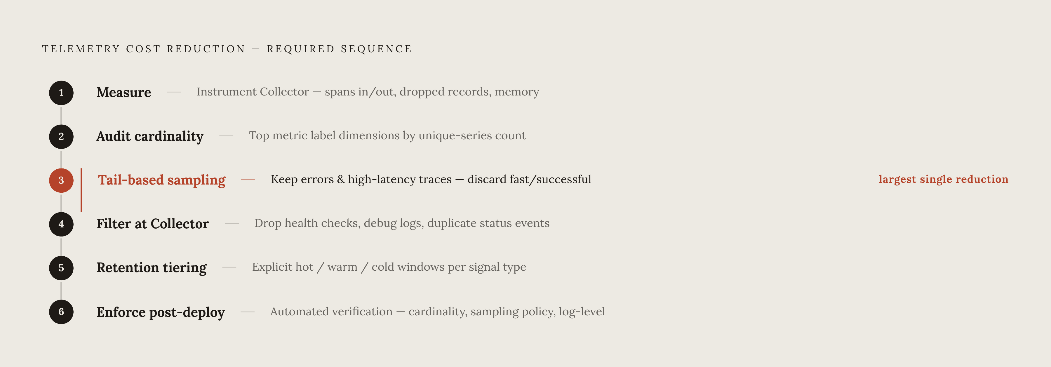
Teams attempting to optimize telemetry cost in all directions simultaneously make no progress. A sequenced approach that addresses the highest-ROI lever first and builds on each win produces faster, more durable results. The order matters.

Step one is measuring before cutting. Instrument the Collector to expose its own internal metrics: spans in, spans out, dropped records, and memory usage. Without this baseline, optimization is guesswork and teams risk cutting data they actually use.

Step two is auditing cardinality. Identify the top metric label dimensions by unique-series count. High-cardinality dimensions that are not actually queried in incident workflows or SLO dashboards are the first targets for removal or Collector-side stripping.

Step three is enabling tail-based sampling. Replace head-based sampling, or no sampling, with tail-based sampling configured to keep 100% of error and high-latency traces. This is typically the single largest reduction in trace storage cost and the step with the clearest tradeoff profile.

Step four is filtering at the Collector before ingest. Add filter processors for known noise sources: health checks, debug log output, and duplicate status events. Start with the highest-volume, lowest-query-rate sources identified in the baseline measurement.

Step five is implementing retention tiering. Define explicit retention windows per signal type and per data class. Hot storage should hold only the window that incident response actually requires.

Step six is enforcing controls post-deploy. Establish automated verification that telemetry pipeline invariants, cardinality ceilings, sampling policy, and log level configurations, hold after every deploy. Treat a violation as a regression, not a billing surprise.

The objection that aggressive optimization sacrifices visibility when it matters most is answered by the sequence itself. Cost discipline is an engineering outcome, not a finance mandate. Teams that instrument deliberately, filter systematically, and verify automatically ship faster because their production signal is cleaner, not just cheaper.